Fixed Distribution
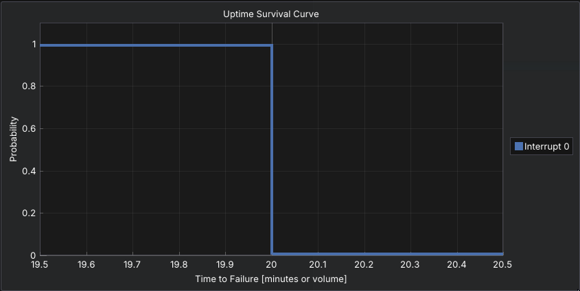
The Fixed distribution always returns the same value. It has no randomness and zero variance, making it useful for modeling predictable, scheduled events such as shift changes, planned maintenance, or regular breaks.
Mathematically, this is a degenerate distribution with all probability mass at a single point. Use it when timing is known and variability is not desired.
Uniform Distribution
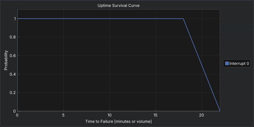
The Uniform distribution selects values evenly between a minimum and maximum, giving every outcome in that range equal probability. It introduces randomness while remaining bounded.
This distribution has constant probability density and moderate variance. It is useful when failures or repairs can occur anywhere within a known range but no particular value is more likely than another—often used when limited data is available.
Normal Distribution
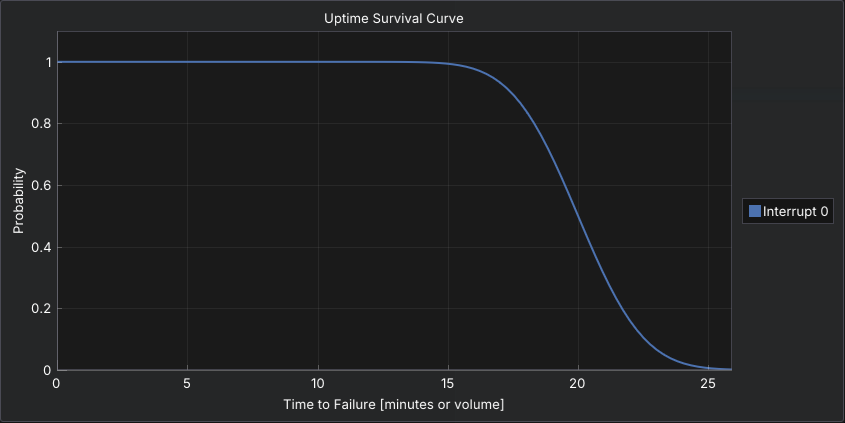
The Normal (Gaussian) distribution produces values symmetrically around a mean, with most outcomes clustering near the average and fewer extreme values.
It is defined by its mean and standard deviation. Normal distributions are useful for modeling naturally varying repair times or human-driven processes, but should be applied carefully to Time to Failure since it allows negative values unless constrained.
Weibull Distribution
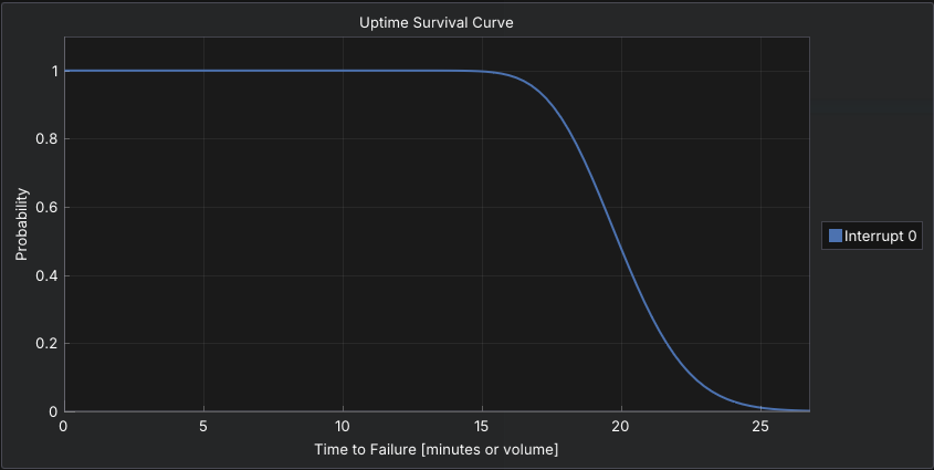
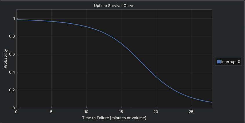
The Weibull distribution is highly flexible and commonly used for reliability modeling. Depending on its shape parameter, it can represent decreasing, constant, or increasing failure rates.
This makes Weibull ideal for modeling wear-out behavior, early-life failures, or aging equipment. It is defined by shape and scale parameters, allowing you to capture a wide range of real-world failure patterns. It has a few key advantages that make it well suited to this type of modeling:
- There is no chance of a negative result. The way a Weibull distribution is constructed, all values below zero have zero probability. This is useful for because it does not allow for the time between two events to be negative, which would be unrealistic.
- By modifying the different parameters, distributions of many different shapes can be achieved. This makes the Weibull extremely versatile in its ability to model all sorts of events.
ChiAha's Weibull distribution uses the two parameter model:
- Parameter 1 is the scale parameter, which represents the spread that 63% of the TTF values occupy.
- Parameter 2 is the shape parameter, which is how the failure rate data is distributed.
Parameter 2 can be interpreted as follows:
- A value less than 1 represents a decreasing failure rate over time. This happens if there are significant pre-mature failures leading to a high probability of failure very early in a cycle.
- A value of 1 shows that a failure rate that is constant over time. This typically suggests random external events are causing interrupts or failures. This reduces the Weibull to an exponential distribution.
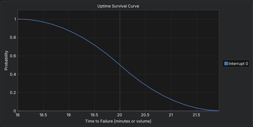
- A value greater than 1 indicates that the failure rate increases with time. This is typically seen as some component of the process changes over time in some way. This could manifest as physical wear or a drift in the process over time that increases the likelihood of failure as time moves on. These are typically described as wear-out failure modes. As the value grows above 1, the Weibull distribution reduces from a lognormal distribution to approaching a normal distribution.
The example below shows the probability density function for 4 Weibull distributions. Each distribution has a parameter 1 value of 1.0 and a range of parameter 2 values from 0.5 to 5.0. This helps illustrate the many different forms that a Weibull can take with parameter modification.
Lognormal Distribution
The Lognormal distribution produces only positive values and is skewed to the right, meaning most values are small with occasional large outliers.
It is often used when failures or repairs result from multiplicative processes, such as compounded delays or variable recovery times. Lognormal is well suited for repair durations or downtime where rare but significant events occur.
Johnson SU Distribution
The Johnson SU distribution is a highly flexible distribution capable of modeling skewed and heavy-tailed behavior. It can approximate many real-world patterns that are not well represented by standard distributions.
Defined by four parameters, it is useful when empirical data does not fit simpler distributions. Johnson SU is typically applied when detailed historical data is available and precise fitting is required.
Exponential Distribution
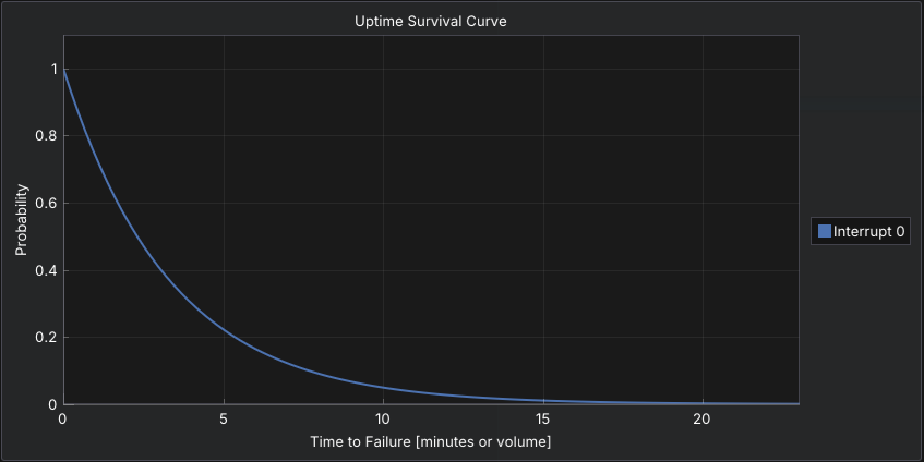
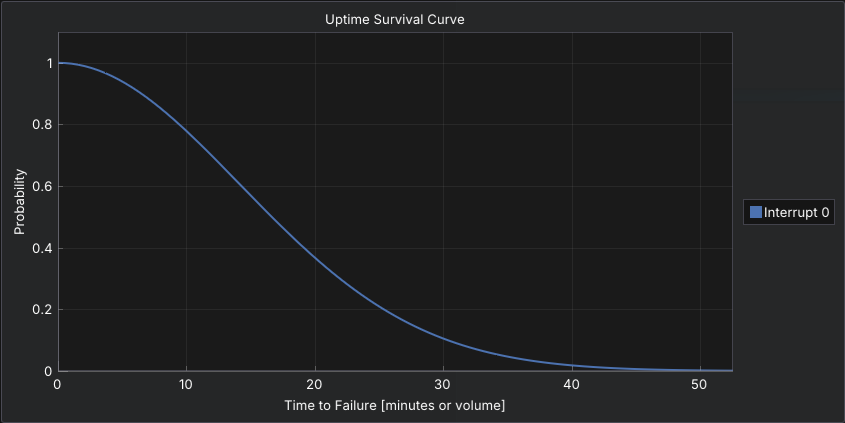
The Exponential distribution models memoryless behavior, meaning the probability of failure does not depend on how long the system has already been running.
It has a constant failure rate and is commonly used for random, independent failures. This makes it appropriate for modeling unpredictable breakdowns where wear does not accumulate.
Triangular Distribution
The Triangular distribution is defined by a minimum, maximum, and most likely value. It provides a simple way to represent uncertainty when limited data is available.
Its piecewise linear shape makes it easy to understand and communicate. Triangular distributions are often used for repair times or downtime estimates when expert judgment provides approximate bounds and a typical value.